Engineers have long understood the benefits of turbulent flow as it applies to heat transfer, and for decades molding experts have talked about the importance of achieving turbulent flow in mold cooling circuits. But what is it about turbulence that makes it so important? What can be measured and demonstrated to have some tangible value to molders? As manufacturers of cooling-related products in this industry, we have a natural curiosity about these questions. Several months ago we began a quest to find some answers.
We elected to do our research with a test mold equipped with electric cartridge heaters. We chose this method because it is much easier and less costly to vary an electric heat source to simulate injection molding than to use an actual press shooting hundreds of pounds of resin. As any experienced molder knows, it can take hours for the mold temperature to stabilize after a process change. Our test mold setup provided a convenient and accurate way to control the variables and replicate the thermal responses of the big hunk of steel in a molding press that we call a mold. Thus, it is a much more user-friendly research tool.
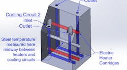
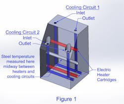
The test mold (Figure 1) is of a size and shape that resembles a small tool that might run in a 100-150 ton press. Two 750W heater cartridges powered by a variable AC voltage source can be cranked up to about 5100 BTU/hr—roughly the equivalent of molding 15.4 lb/hr of nylon 6 at 570°F melt temperature. The test mold has two 7/16-in. ID cross-drilled, U-shaped cooling loops of different lengths. We can use either or both cooling circuits and they can be plumbed in parallel or series. The inside walls of these circuits were clean and smooth. A temperature sensor was placed strategically between the heaters and the cooling loops to study the temperature response of the steel to variations in cooling conditions for a given heat input.
Coolant flow and temperature were monitored and recorded to a suitable level of accuracy. The temperature change (ΔT) of the coolant moving through the mold becomes small as flow increases so those temperature measurements must be very accurate and repeatable. Water inlet and outlet temperature were measured with a matched pair of laboratory-grade RTD sensors and readers that produce results consistent within 0.1°C.
Flow measurements were made with our NIST-traceable flow calibration system, more accurate than necessary, but convenient for us to use.
To date, we have conducted experiments with a single cooling circuit and with two circuits plumbed both in parallel and in series. The coolant is local tap water with treatments to control pH and biological agents. Trial runs were conducted at a fixed power input while coolant flow was varied from substantially below to well above the turbulent range. After each change in flow rate, sufficient time was allowed for the steel temperature to stabilize, sometimes taking as long as 3 hr. Coolant inlet and outlet temperatures, flow rate, and steel temperature were all recorded throughout the flow range.
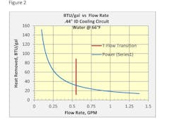
The data collected in our numerous trials allowed us to calculate accurately the temperature change (ΔT) of the coolant as it passes through the mold. Knowing ΔT we could calculate the BTUs removed by each gallon of water. We plotted BTU/gal against flow rate (Figure 2). This chart shows clearly that BTU/gal decreases as flow-rate increases, even as the flow transitions to turbulent. We were surprised by this result, but the math shows us that we should have expected it. Heat transfer is based simply on the increase in water temperature: BTU/gal = ΔT x (1 BTU/lb-°F) x 8.3 lb/gal
The faster the water goes through the mold, the less the temperature increases. This result leaves us still wondering: Where is the “magic” of turbulence?
We believe our data sheds some light, but we had to think in a different way. But before we get to that, let’s back up and think about what molding cooling is really about. What is it that we really need to accomplish? The real objective is to control the cooling rate and temperature of the parts so they can be ejected at the earliest possible time while maintaining the desired properties and dimensions. Today’s process monitoring and control technology is highly advanced and sophisticated, but to imagine directly controlling the part temperature in the mold is still science fiction. So we do the next best thing— we try to control the temperature of the mold, thereby indirectly controlling part cooling.
Now let’s think of the mold as a very strange kind of heat exchanger. Molten plastic supplies heat to the mold and the coolant takes the heat away. However, there are some key differences between our mold/heat exchanger and a conventional heat exchanger.
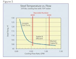
One is that we are trying to control the temperature of the body of our heat exchanger (the mold). Two, our heat exchanger is a large mass of metal with a very slow temperature response. Think of it as a big thermal flywheel. Any “normal” heat exchanger has certain performance characteristics related to inlet and outlet conditions for both fluids. The heat transfer performance of a mold is revealed by plotting steel temperature (measured at a strategic point) vs. coolant flow rate (Figure 3).
It is true that there are endless sizes of molds with endless different heat inputs and cooling schemes, and each one will have its own unique response to the thermal inputs and cooling system. For each one, it would be possible to create a graph of mold temperature (measured at a meaningful point) vs. coolant flow rate—a heat-exchanger performance curve. We believe this curve shows us something interesting about turbulence and efficient mold cooling. For that reason, we decided to call it the “Value Curve.”
Here is what we believe the Value Curve tells us: The vertical axis represents steel temperature and the horizontal axis represents the water flow rate. The distinctive L-shaped curve is defined by low flow and a nearly vertical leg at the left and by higher flow toward the right as the curve becomes more horizontal.
Note that the transition to a more horizontal shape occurs around the predicted turbulent flow rate. The steep curve shows a large change in steel temperature resulting from a very small change in flow rate. The more horizontal portion of the curve shows a range where steel temperature changes only slightly as flow increases substantially. You could say that at flow values well below turbulence, steel temperature is less stable, changing significantly with small changes in flow rate. In contrast, after the transition to turbulent flow the curve flattens out and steel temperature changes little with increasing flow—in other words, it becomes more stable.
You might also conclude that increasing flow to well above turbulence yields little additional benefit and is costly in terms of flow capacity. Thus, the Value Curve suggests that operation with coolant flow slightly above the turbulent rate offers stable and economical operation and that substantially higher coolant flow might be considered wasteful.
